
2. Pipelining
2장 Pipelining 개요
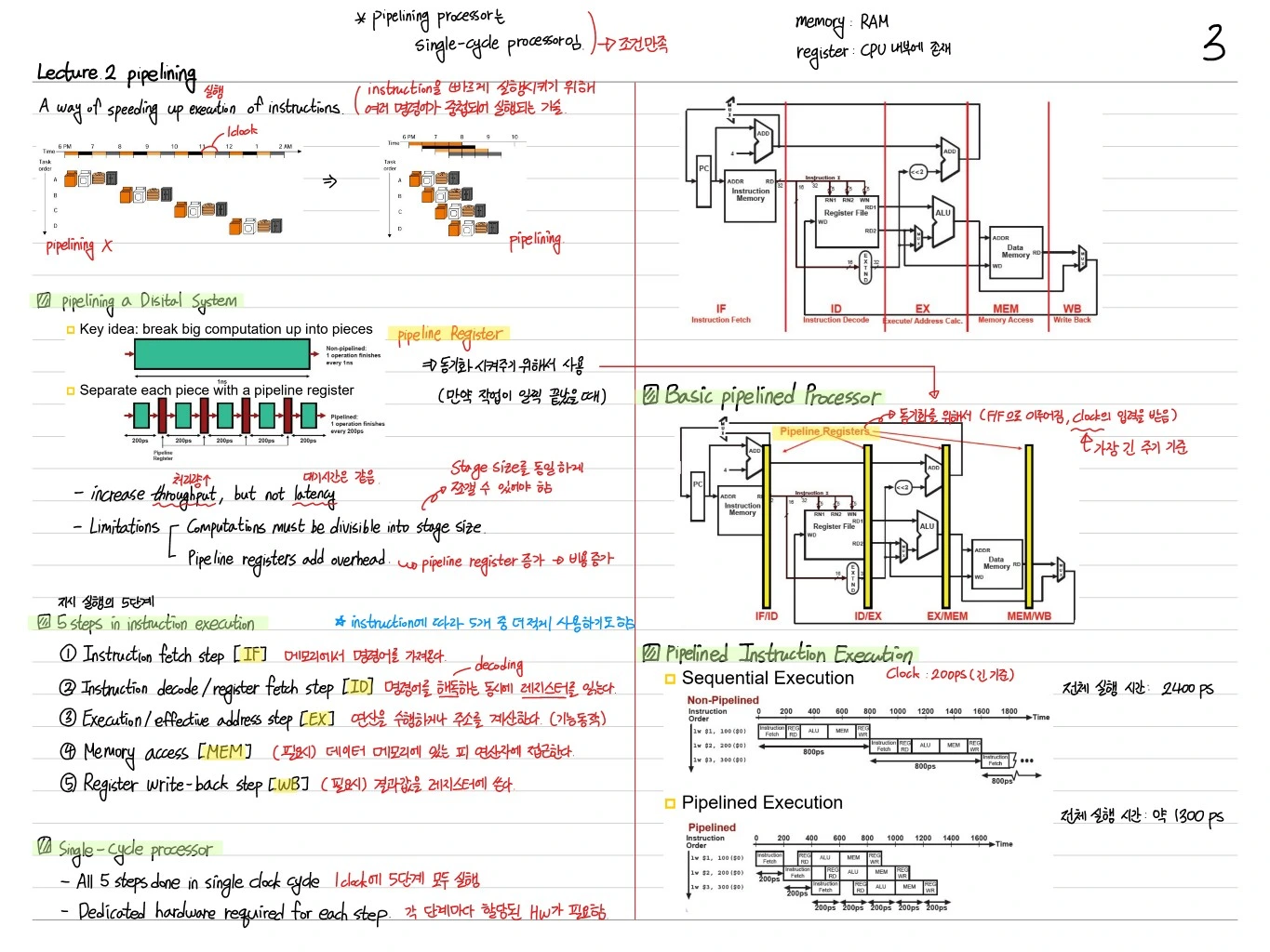
Pipelining은 명령어 수(= number of instructions)가 아닌 실행 속도를 높이는 기술이다. 하나의 명령어 처리를 여러 stage로 나누고, 각 stage를 독립적으로 병렬 실행해 처리량(throughput) 을 높인다.
Pipelining in Ordered System
pipelining의 핵심 아이디어: 일을 단계별로 쪼개고, 각 단계는 pipeline register에 의해 격리되어 동시에 서로 다른 명령어의 다른 단계가 수행된다.
- Advance physical, but not latency
- Limitation: 단일 작업의 latency는 줄어들지 않음
- Pipeline stage은 가장 느린 stage에 의해 결정됨 (slowest stage가 전체 clock period를 결정)
5-Stage MIPS Pipeline
MIPS pipeline은 보통 5단계로 구성된다.
- IF (Instruction Fetch) — 메모리에서 명령어 읽기
- ID (Instruction Decode + Register read) — 디코딩 & 레지스터 읽기
- EX (Execute) — ALU 연산
- MEM (Memory access) — load/store 시 메모리 접근
- WB (Write Back) — 레지스터에 결과 기록
Sequential vs Pipelined 성능 비교
동일한 명령어를 실행할 때:
- Sequential Execution: 각 명령어를 모든 stage 완료 후 다음 명령어 시작 (예: 8ns × 3 instructions)
- Pipelined Execution: 각 stage가 겹쳐서 실행 → 전체 시간이 2ns × (3 + 4) = 약 14ns로 단축
즉 명령어 수가 많을수록 이상적으로는 stage 수만큼 throughput 증가.
Hazards — 파이프라인의 적
Pipeline이 이상적으로 동작하지 않도록 막는 hazard 세 종류:
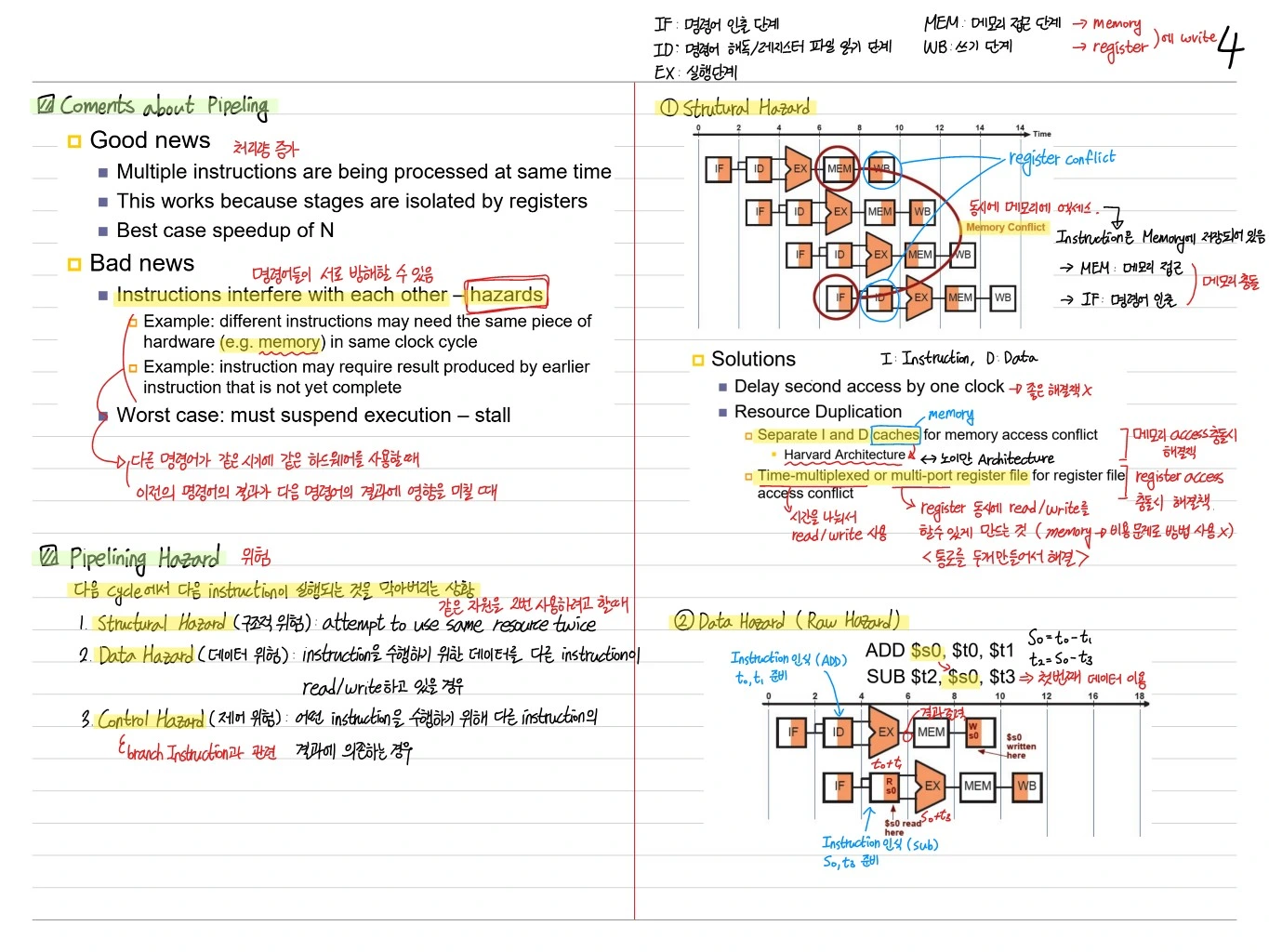
1. Structural Hazard
Multiple instructions are being processed at same time.
예: 하나의 메모리를 IF와 MEM이 동시에 쓸 때 충돌. → Solutions:
- Replicate resources (I-cache / D-cache 분리)
- pipeline register로 stage별 격리
2. Data Hazard
이전 명령어의 결과를 다음 명령어가 사용해야 하는 경우.
예:
add r1, r2, r3    # r1에 값을 쓰고
sub r4, r1, r5    # 바로 r1을 읽음 → r1 아직 WB 안됨
이전 명령어가 아직 WB 단계에 도달하지 않았을 때 뒤 명령어가 읽으면 잘못된 값을 가져감. Worst case: suspend execution — stall.
Solutions
- Delay second access — 이전 명령어 결과가 도착할 때까지 정지 (stall / bubble)
- Resource Duplication
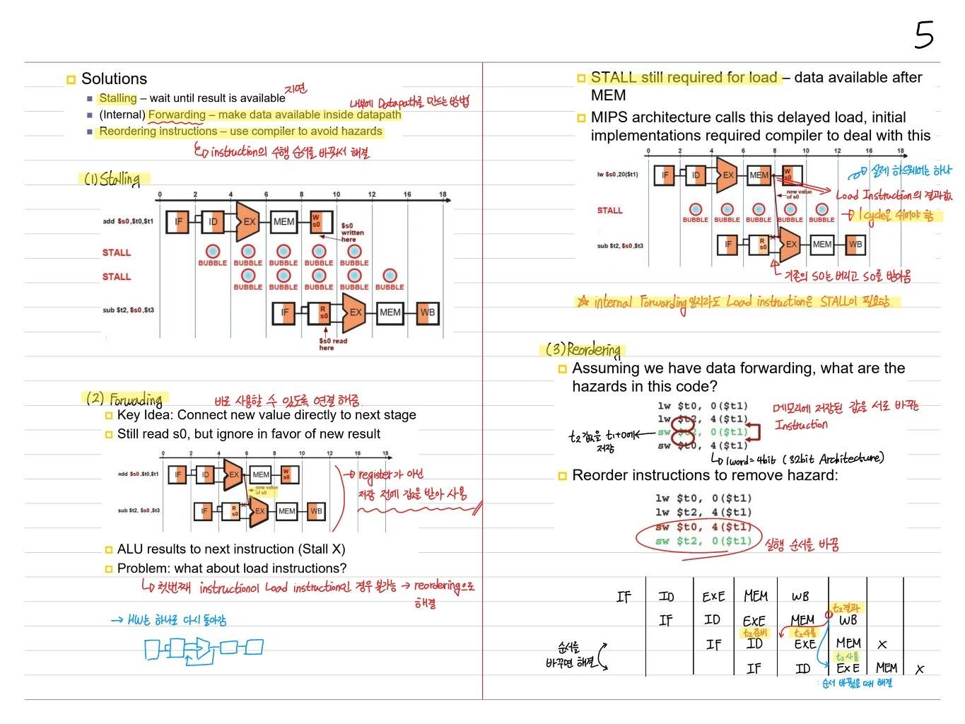
- Forwarding (Bypassing): ALU 결과를 WB 대기하지 않고 곧바로 EX 입력으로 전달. Pipeline register에서 다음 stage로 직접 연결.
Load-Use Data Hazard
Forwarding으로도 해결 안 되는 경우: Load 후 바로 그 값을 사용하는 경우. Load의 값은 MEM stage 끝에 나오므로, 다음 명령어의 EX 전에 도달 못 함 → 1 cycle stall 필수.
MIPS architecture calls this delayed load, initial implementations required compiler to deal with this.
Stall / Bubble
- Key idea: Connect new value directly to next stage
- Still need to stall for stalls → load instruction의 load-use 해결
- ALU results to next instruction (Stall X)
- Problem: what about load instructions? → 다음 명령어 stall + forward
3. Control Hazard (Branch Hazard)
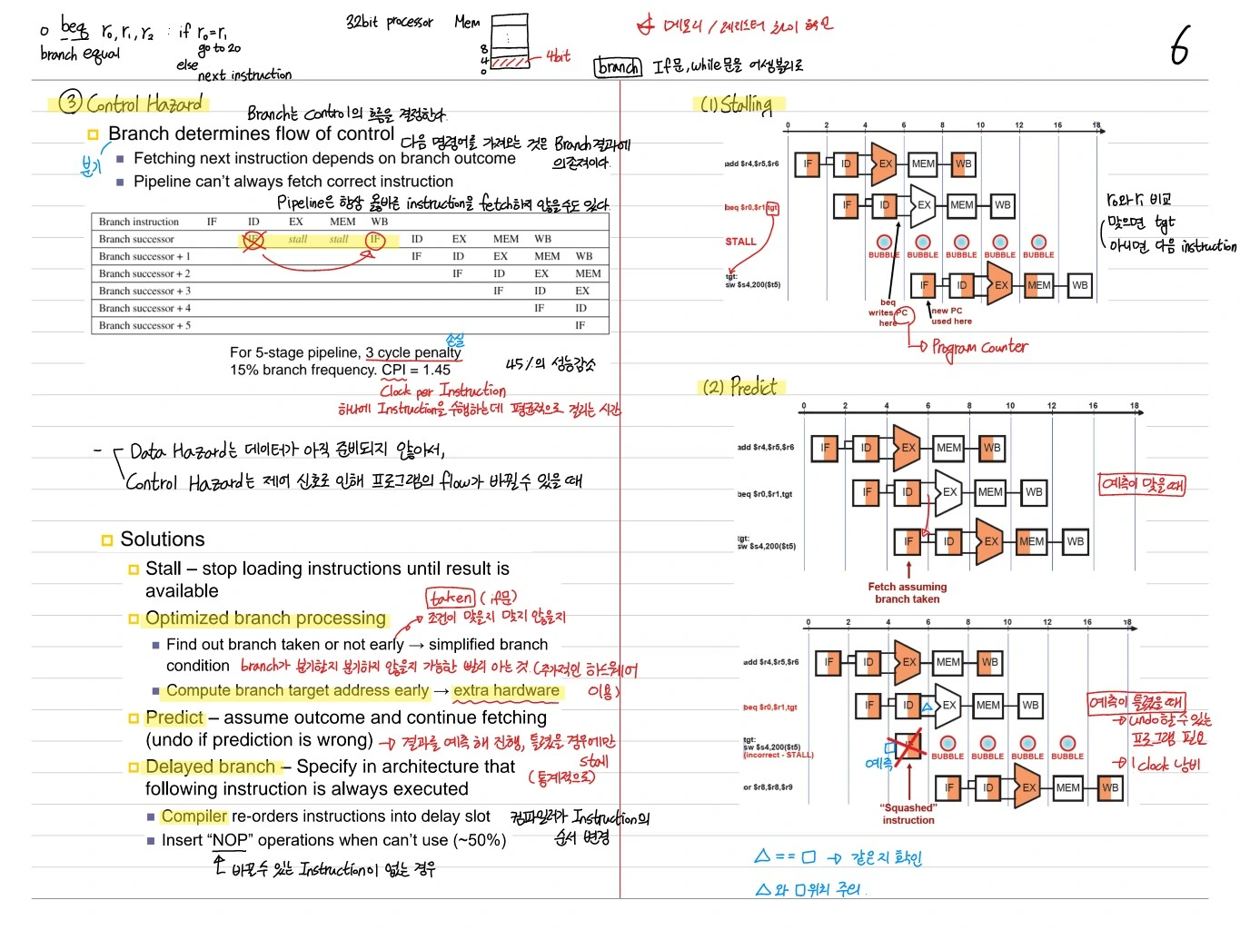
Branch determines flow of control. 분기 결과가 확정되기 전에 뒤 명령어를 fetch하면, 잘못된 명령어를 실행할 수 있음.
- Pipeline can''t always fetch correct instruction — fetch 단계에서 PC를 결정해야 하는데 branch는 EX 전에 확정되지 X
- 5-stage pipeline, branch 10% 기준 branch penalty:
$$\text{CPI} = 1 + 0.1 \times 3 = 1.3$$
→ 10% branches × 3 cycle stall = 15% branch impact → MIPS가 20% 성능 저하
Solutions
- Stall — 단순하지만 loading instructions until result is available
- Compromise branch processing — simplified branch condition
- Prediction — assume outcome and continue fetching (predict not-taken → flush if wrong)
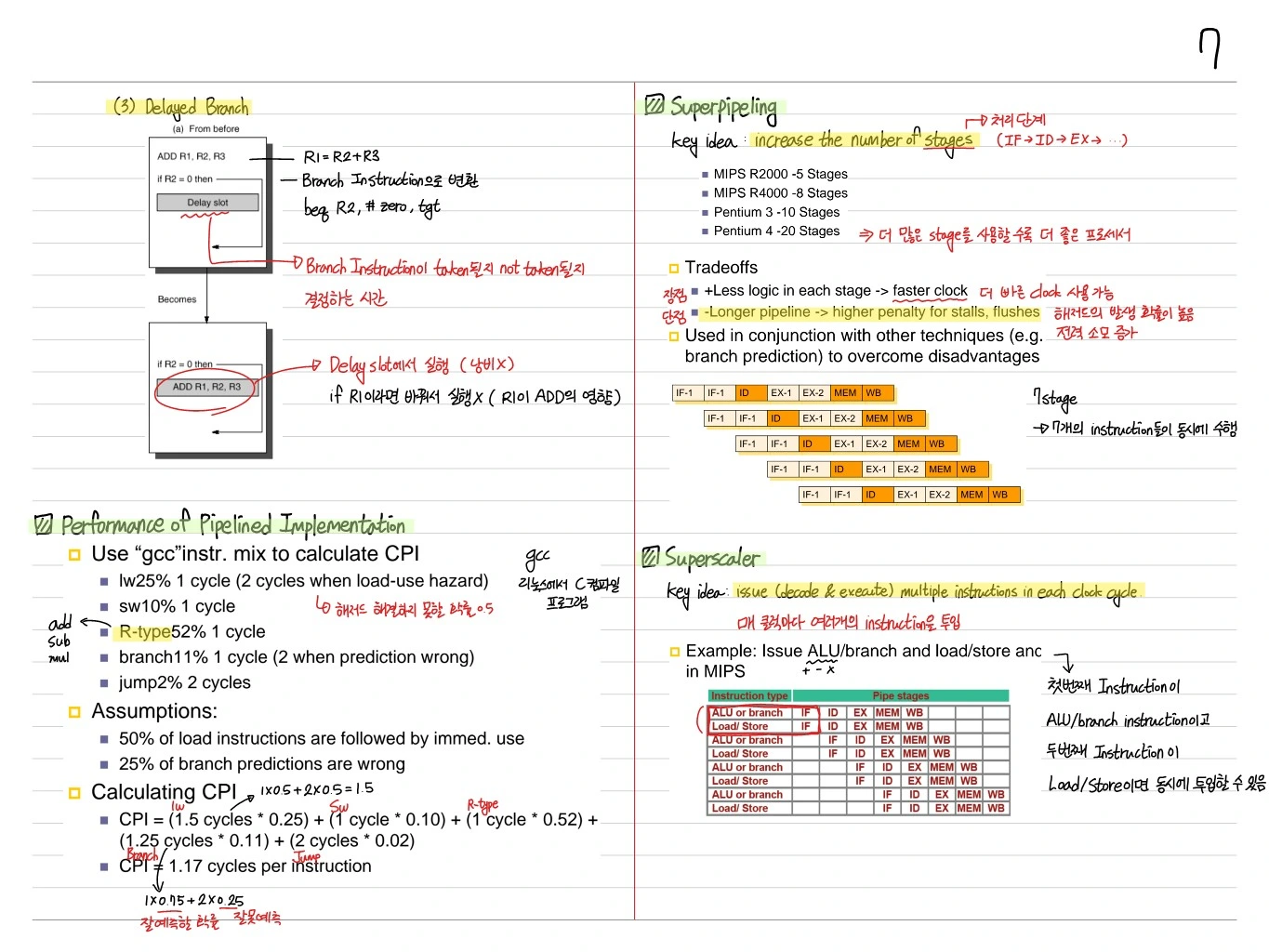
- Delayed branch — compiler schedules a useful instruction into the delay slot (MIPS)
- Compile re-orders instructions into delay slot. Insert
nop(no operation) instructions when can't reorder.
Pipelined Implementation의 성능
CPI 계산 예
- Use "gcc" instruction mix to calculate CPI
- IW = 25% (2 cycles when load-use happen)
- SW = 10% (1 cycle)
- R-type = 52%
- Branch = 11% (1 cycle delayed branches)
- Jump = 2% (1 cycle)
가정: 50% of load instructions are followed by immed. use.
$$\text{CPI} = 0.5 \times (0.25 \times 2 + 0.75 \times 1) + 0.5 \times (0.25 \times 0.52 + 0.10 \times 0.11 + 0.02) = \text{약 } 1.17$$
→ Pipelining 덕분에 1.17 cycles per instruction의 효과.
Superpipelining
Key idea: Increase the number of stages. 예: Pentium 4 → 20 stages.
- Advantages: Faster clock (각 stage 짧음)
- Disadvantages: Longer pipeline → higher branch penalty, flush 많음
- Used in conjunction with other techniques to overcome disadvantages (branch prediction)
Superscalar
Key idea: Issue (and execute) multiple instructions in each clock cycle.
Example: Issue ALU/branch and load/store at MIPS:
| ALU / branch | Load / Store |
|---|---|
| nop | lw $t0, 0($s1) |
| add $s1, $s1, $s0 | sw $t0, 0($s1) | |
| nop | ... |
→ 복수 instruction을 동시에 issue. 단 dependency 지키기 위한 scheduling 복잡.
Software Manipulation to Increase ILP
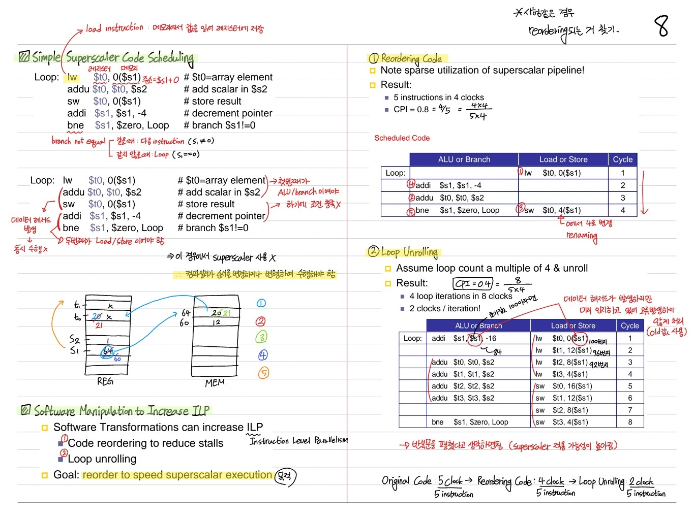
Simple Superscalar Code Scheduling
Loop:
  lw   $t0, 0($s1)   # $t0 = array element
  addu $t0, $t0, $s2 # add scalar in $s2
  sw   $t0, 0($s1)   # store result
  addi $s1, $s1, -4  # decrement pointer
  bne  $s1, $zero, Loop  # branch $s1 != 0
Reordering — 의존성 없는 명령어 재배치
Note: Update value of $t0 will not be available for next iteration → 의존성 있는 instruction들을 멀리 배치하면 stall을 피할 수 있다.
Loop Unrolling
Assume loop count is multiple of 4, & unroll 4 loop iterations in 4 cycles.
Loop:
  lw $t0, 0($s1)   lw $t1, -4($s1)
  lw $t2, -8($s1)  lw $t3, -12($s1)
  addu $t0, $t0, $s2  addu $t1, $t1, $s2
  ...
→ Superscalar에서 4 × IPC = 4 cycles per 4 iterations (이상적)
Dynamic Pipeline Scheduling
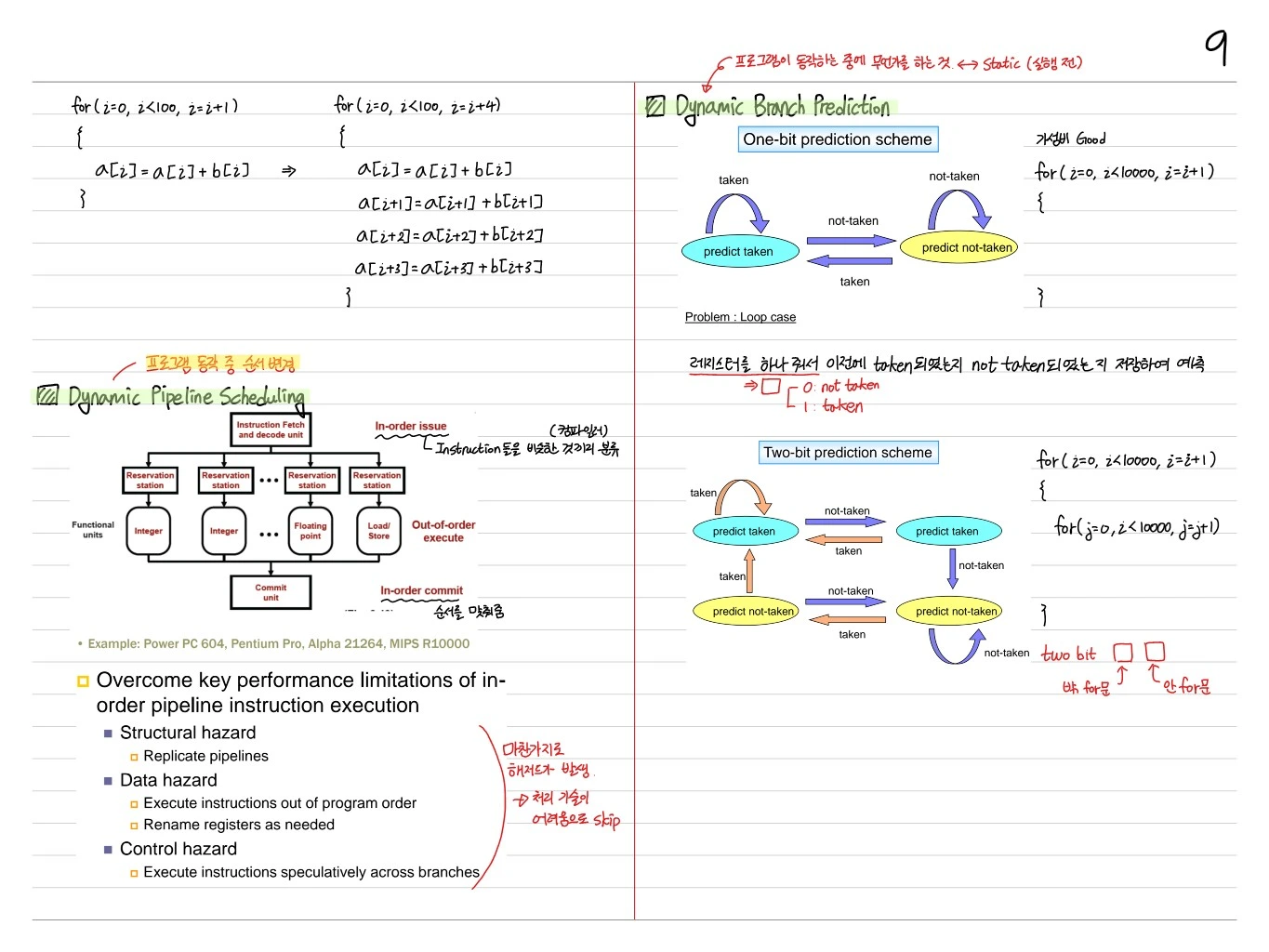
프로그램이 동작 중 명령어들의 순서를 동적으로 변경하는 기법. 컴파일러가 아닌 하드웨어가 수행.
Out-of-order Execute, In-order Commit
Instruction Fetch & Decode unit (In-order issue)
         │
   ┌─────┼─────┬─────┬─────┐
   ▼     ▼     ▼     ▼
 Reservation stations (× N)
   │     │     │     │
   ▼     ▼     ▼     ▼
Integer  Integer  Floating point  Load/Store
   │     │     │     │
   ▼     ▼     ▼     ▼
   Commit unit  (In-order commit)
- Example: Power PC 604, Pentium Pro, Alpha 21264, MIPS R10000
- Reservation station에 instruction을 비슷한 것끼리 분류(컴파일 순서 아님)
- Out-of-order execute → 처리 가능한 것부터 먼저 실행
- Commit은 순서를 맞춰서 in-order
Overcomes Key Performance Limitations
- Structural hazard → Replicate pipelines
- Data hazard → Execute instructions out of program order, Rename registers as needed
- Control hazard → Execute instructions speculatively across branches (투기적 실행)
처리 가중치가 어려운 것부터 skip 가능 → stall 감소.
Dynamic Branch Prediction
프로그램이 동작하는 중에 분기를 예측하는 것 (↔ Static은 실행 전).
One-bit Prediction Scheme
- 각 branch에 대해 이전에 taken됐는지 not-taken됐는지를 한 비트로 저장해서 예측
- 예:
for (i=0; i<10000; i++)같은 루프는 Good (대부분 taken) - Problem: Loop case (마지막 iteration에서 잘못 예측)
레지스터를 하나 줘서 이전에 taken됐는지 not-taken됐는지 저장하여 예측.
Two-bit Prediction Scheme
state machine: predict taken / not-taken 두 상태가 아니라 4 상태 (strong taken, weak taken, weak not-taken, strong not-taken).
- 한 번 틀려도 바로 예측 뒤집지 않음 → Loop case에서도 정확도 높음
- Nested loop에서 안 for문 / 바깥 for문 모두 잘 예측
for (i=0; i<10000; i++)       ← 바깥
  for (j=0; j<10000; j++)     ← 안쪽 (taken이 더 많음)
정리
| 기법 | 목적 | 대표 예 |
|---|---|---|
| Pipelining | Throughput ↑ | 5-stage MIPS |
| Forwarding | Data hazard 최소화 | EX → EX bypass |
| Delayed branch | Control hazard 완화 | MIPS 1 cycle delay slot |
| Superscalar | IPC ↑ | Pentium Pro |
| Superpipelining | Clock ↑ | Pentium 4 (20 stages) |
| Out-of-order | 하드웨어 스케줄링 | R10000, Alpha 21264 |
| Branch Prediction (2-bit) | 분기 정확도 ↑ | 현대 CPU 표준 |
pipelining과 그 변형들은 하드웨어 병렬성의 기본이고, 이후 캐시 계층, virtual memory, multi-core까지 이어지는 토대가 된다.
 Computer Architecture Note
 AI Study Note
 Embedded Note
 SoC Note
Comments (0)
No comments yet. Be the first to comment!
Please to write a comment.